Mapping and Simulation
The Mapping workspace in Fulcrum One allows for fast, powerful real-time coverage prediction of loudspeakers and loudspeaker systems in room models. Loudspeakers may be rapidly moved, aligned, and processed, and their associated performance updated on a spatial coverage map in real-time, allowing for an extremely efficient design workflow.
Note: Coverage mapping in Fulcrum One currently predicts the free-field, direct sound contribution of loudspeakers in the model at surfaces and measurement "probes". Time-domain / phase interference and air loss over distance is fully modeled, as is basic shadowing for line-of-sight occlusion (diffraction is not modeled).
Parameters that include room acoustics and ambient noise level assume these acoustic fields to be fully diffuse and uniform in nature.
To begin mapping a system, make sure you've selected the Mapping workspace using the tab at the top of the window.

Preparing the Model
To map loudspeaker coverage in a model, we need to enable model surfaces to receive and display energy from the loudspeaker system. You can enable any 3D model surface as a mapping plane in your project. Obviously, audience areas are of primary importance, however, you can also easily enable things like stage surfaces or walls to see how much energy is being projected onto those areas.
To enable a surface, click the surface in your 3D model. In the Properties toolbox, enable mapping on that surface using the  control. The model will immediately add that surface to the visualization. Alternately, you may right-click the surface and check Mapping in the context menu.
 control. The model will immediately add that surface to the visualization. Alternately, you may right-click the surface and check Mapping in the context menu.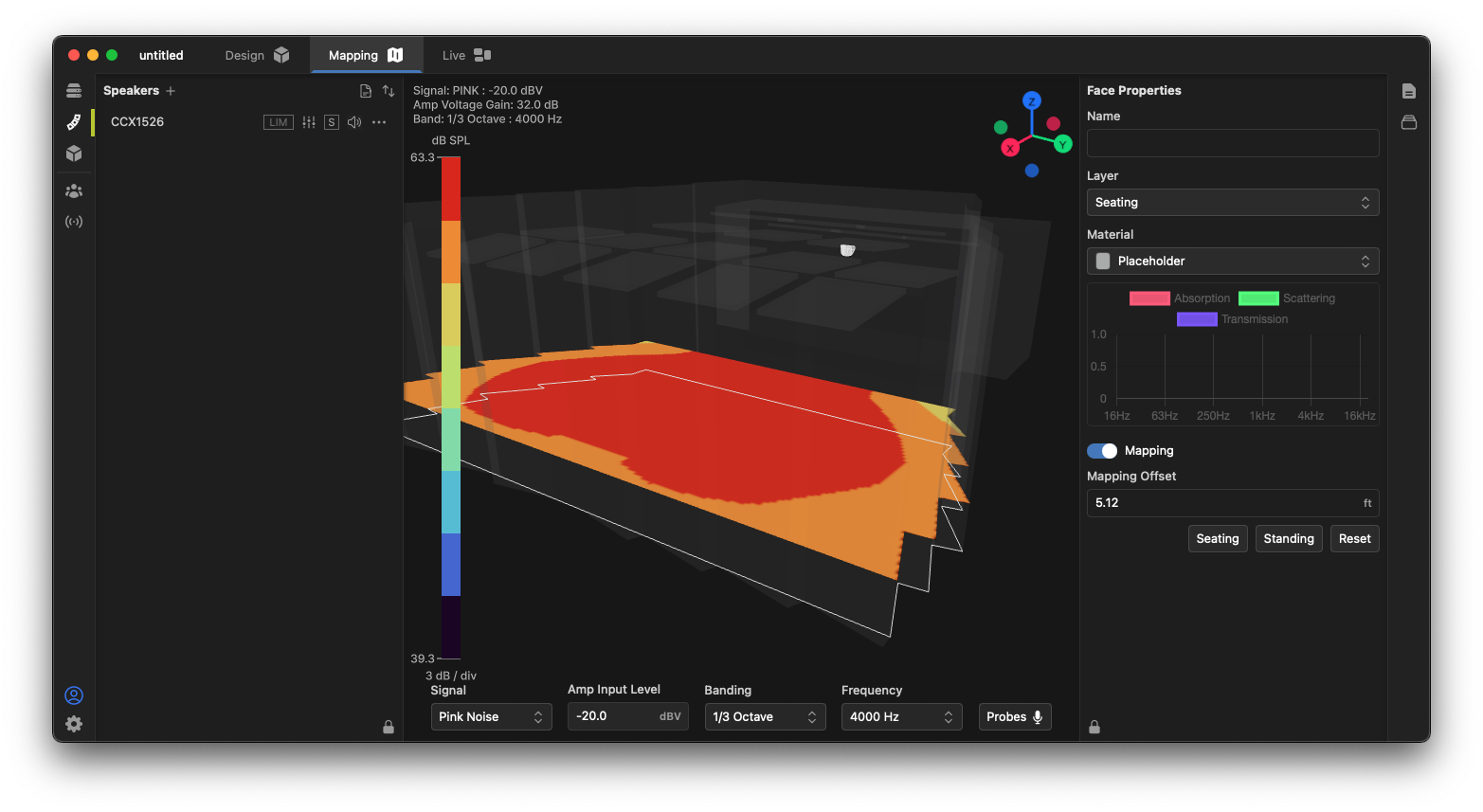
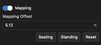
By default, an enabled surface calculates and displays the mapping data in the same plane as that surface. You can, however, offset that mapping to a distance away from the plane. This is useful for drawing improvised audience planes above, for example, a floor-level surface in a model. In the Properties toolbox, enter the offset height as a number, or click the Seating or Standing presets to create an offset equal to a standard seated or standing ear height.
Mapping Controls
The Mapping toolbar allows you to quickly change what you are simulating without leaving the 3D view. Every control updates the map and any open probes in real time.
Reading the bar from left to right. Control labels appear when you hover over each button in the toolbar:
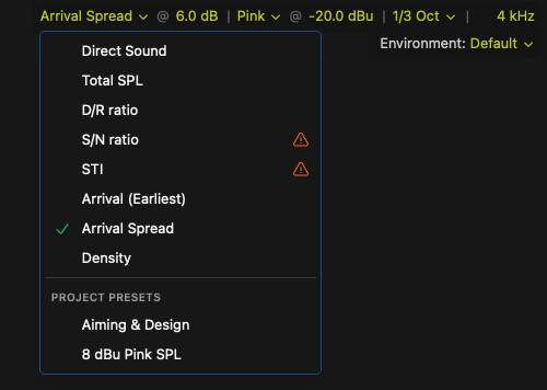
- Mode — selects the active simulation mode (Direct Sound, Total SPL, D/R ratio, S/N ratio, STI, Arrival (Earliest), Arrival Spread, or Density). Modes that require a configured environment display a warning icon when one is missing.
- @ x dB — the SPL threshold for threshold-based modes. In Arrival (Earliest), Arrival Spread, and Density, only loudspeakers whose level is within this many decibels of the loudest arrival at each point are counted. This control is hidden for modes that do not use it.
- Signal — the source signal used to drive the system. Available options include:
- Pink Noise: A broadband pink noise signal with equal energy per octave.
- EIA-426B: A broadband noise signal weighted according to the EIA-426B standard, typical for testing loudspeaker SPL capabilities.
- Speech: A male speech signal, typically used for testing speech intelligibility or speech system output capability. This signal follows the standard STI test signal according to IEC 60268-16:2020. STI calculations always utilize this test signal.
- Music Noise: A broadband noise signal with RMS spectrum weighted according to the AES75-2023 standard, typical for testing music system output capability.
- @ x dBu — the amplifier input level RMS voltage level, referenced to 0.775 V. Together with the amplifier voltage gain, this sets the drive level used to calculate SPL.
- Banding and frequency — the analyzer resolution (Broadband or fractional-octave such as 1/3 Oct) and, when a band is selected, the center frequency being displayed. Click the frequency display to open a slider that allows you to adjust the center frequency.
- Environment — the environment whose room acoustics and noise level are applied to the room-dependent modes.
The remaining analyzer, display, and amplifier settings (weighting, color mapping, dynamic range, contours, mapping grid resolution, and shadowing) live in the settings popover opened from the gear icon.
Project Presets
Project presets save a complete combination of mapping mode and analyzer/signal/display settings under a name so you can switch between common evaluations with a single click. Every new project ships with two built-in presets that you are free to edit, duplicate, or delete:
- Aiming & Design — a Direct Sound preset with a 24 dB contoured scale, tuned for dialing in loudspeaker placement, splay, and coverage.
- 8 dBu Pink SPL — a broadband Direct Sound preset driven with pink noise at 8 dBu for evaluating system SPL capability.
Presets appear beneath the built-in modes in the Mode menu (and in the equivalent menu on each probe tab). You can create new presets after modifying any mode, and manage presets using the Settings menu on the Mapping tab.
Mapping Settings
The calculation and visualization of mapping results is widely customizable using the Settings  menu. This includes customizing the simulated amplifier and input levels, changing weighting, banding and center frequency settings, and customizing the mapping rendering itself.
 menu. This includes customizing the simulated amplifier and input levels, changing weighting, banding and center frequency settings, and customizing the mapping rendering itself.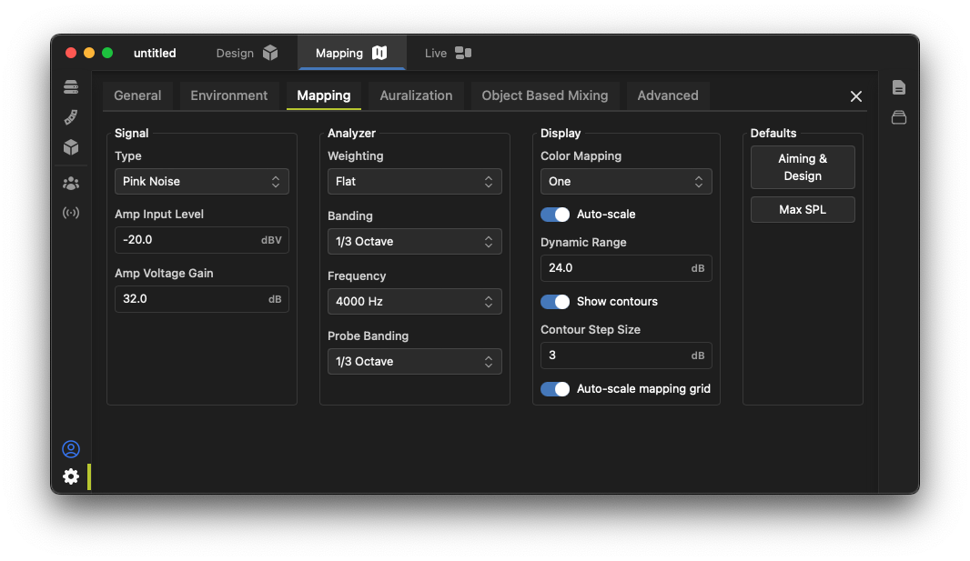
Mapping settings can be saved as "Project Presets" inside the current One file, letting you distribute specific mapping views to others or save them for future use. In addition, you may use the arrow buttons to save or load presets to and from the "User Presets" list, which is saved locally to your computer. In this way, your favorite settings can be quickly and easily applied to new projects.
Aiming and Design
In the Mapping toolbar, click the Aiming & Design preset.
The display will show a mapping of the current system state, usable for judging high frequency coverage throughout the venue.
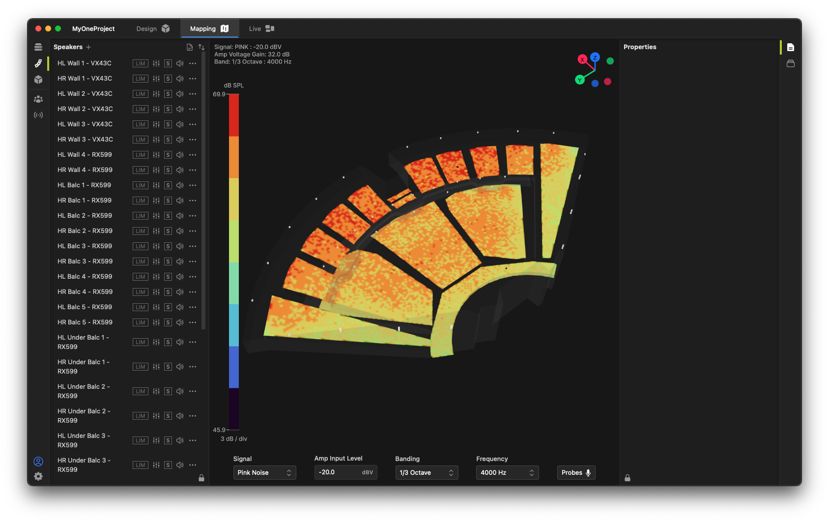
You can quickly and easily change the excitation signal, the simulated input signal level, and the banding & center frequency of the simulation using the controls in the mapping toolbar. Individual speakers can be controlled from the Speaker toolbox. It is typically helpful to selectively mute or solo loudspeakers to help with adjusting individual loudspeakers.

Solo an individual speaker to see its contribution to the venue coverage.
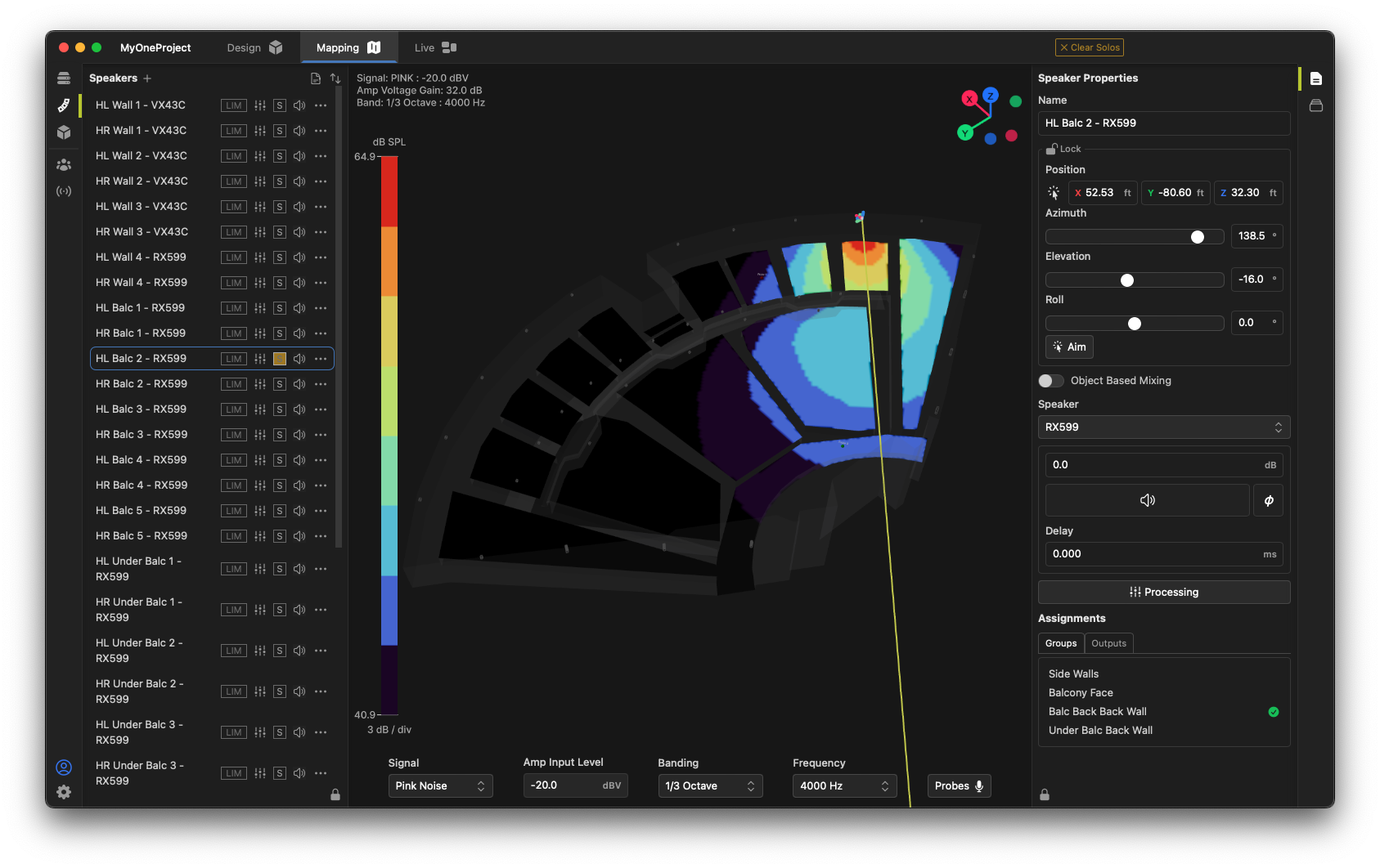
Just like in the Design workspace, you can select a loudspeaker and quickly move or position it using its Properties toolbox. In addition, the position  and aiming
  tools are also available in Mapping workspace.
 and aiming
  tools are also available in Mapping workspace.
Note that speaker groups, speaker signal processing, gains and delays all affect the mapping results, so a processed system can be realistically modeled in the venue. Levels and filters can be "roughed in" and quickly equated to real DSP when the system is implemented.
The headroom available for an individual loudspeaker with the current signal settings can be viewed by hovering over the  indicator in the Speakers list. Above its rated output, a simulated speaker will "limit" and gain reduction will be shown.
 indicator in the Speakers list. Above its rated output, a simulated speaker will "limit" and gain reduction will be shown.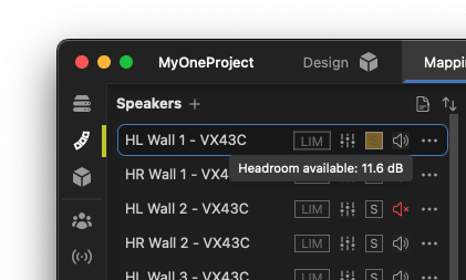
Max SPL
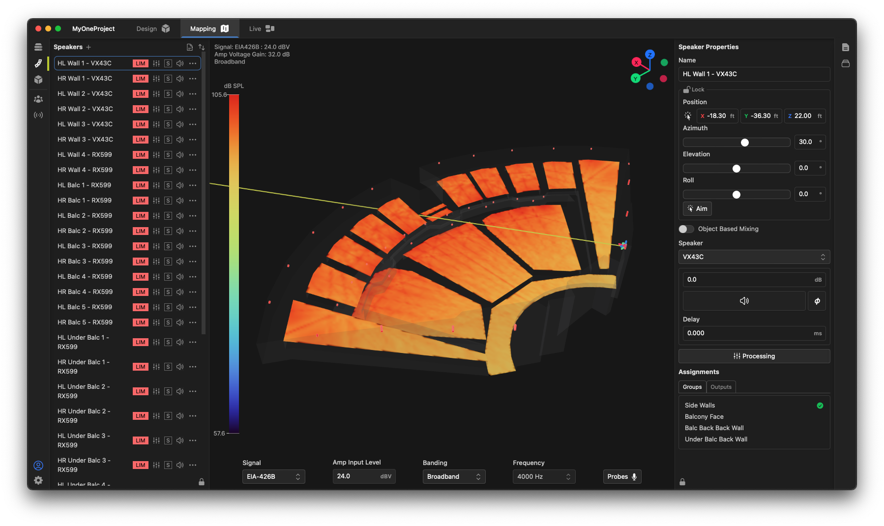
To display the theoretical maximum SPL performance of a system, click the 8 dBu Pink SPL preset in the mapping toolbar.

In this preset, a simulated pink noise signal is driven into the amplifier at 8 dBu, which is the typical maximum input level for all Fulcrum loudspeaker presets with Driveflex amplifiers. This can be easily changed by the user. The coverage map shows the theoretical maximum with all speakers driven to their individual limits on a broadband basis.
Data Readouts
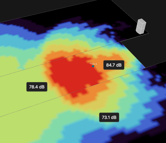
Hovering the mouse over the mapping area will display a readout of the mapped level at that location, reflecting the level shown on the mapping color scale. You can "drop" multiple temporary readouts on the screen by holding the ALT key (Windows) or the Option key (MacOS) while clicking on the surface. Design or processing parameters may be changed and the results seen on the respective readouts. To remove all readouts, hit the ESC key.
Probes
Probes are listening positions you place in the model to inspect the system response at a specific point. The probe tray allows you to organize many probes, compare results, and listen to your design. Click the  icon on the bottom-right of the main window to open the probe tray.
 icon on the bottom-right of the main window to open the probe tray.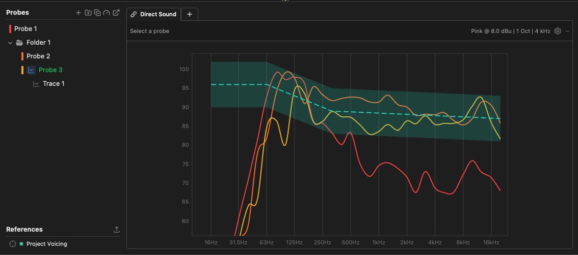
To add a probe, click the + button in the Probes window, or right-click on any mapping surface and select Add Probe. The probe may be easily positioned using the function in the Probe Properties toolbox. Multiple probes may be added to compare the system behavior at different locations.
Organizing Probes
Probes may be organized to help you manage your probes and compare results.
- Folders — group related probes (for example, by seating section or zone). Toggling a folder active or inactive shows or hides every probe inside it on both the map and the chart.
- Traces — capture the current response of a probe as a saved snapshot. A trace remembers the mapping mode and settings it was taken with, so you can store a "before" curve and overlay it against the live "after" response while you make changes. Expand a probe in the list to see its traces.
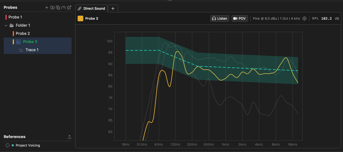
- References — overlays that are not tied to a single probe. Project Voicing plots the project's voicing target so you can compare a measured probe against your intended response. You can also Import an external trace or a target curve into the References list. Imported files follow the Smaart standard for reference curves.
Use the toolbar buttons at the top of the tray to add a probe, add a folder, duplicate, import/export, and pop the tray out into its own window. Probe responses can be exported for use elsewhere, and the gauge button toggles a Direct SPL readout next to each probe in the list.
Comparing Modes with Tabs
The chart area supports multiple tabs. The first (linked) tab always follows the mapping mode selected in the main window. Add additional tabs to pin a probe to a different mode, letting you watch—for example—Direct Sound and STI for the same probe side by side. Selecting several probes overlays their responses on the chart and shows max / average / min statistics in the header.
The chart adapts to the active mode: a frequency-response plot for SPL and ratio modes, an echogram for the arrival and density modes, and a bar graph for STI. To compare multiple probes at once, click into the 3D mapping view so it has focus and deselect any single probe in the tray—when one probe is selected, the chart highlights only that probe's trace.
Listen and POV
When a single probe is selected, two actions appear in the probe header (and on the right-click menu):
 auralizes the design from that probe's position over headphones using Room Auralization, so you can hear what the system sounds like at that seat.
 moves the 3D camera to the probe's point of view, giving you a listener's-eye view of the system. The listener position and orientation can also be moved manually by clicking and dragging in the 3D view—head tracking is optional, not required.
Simulation Modes
In addition to the previous Direct-Sound SPL mapping capability that Fulcrum One has included in previous versions, this version of One includes a number of additional acoustical simulation modes to assist in the design of an audio system to your specifications and expectations.
| Type | Mode | Application | Probe Display |
|---|---|---|---|
| SPL and coverage | Direct Sound | Identical to previous versions, this mode shows the direct sound incident on the mapping area or probe with no influence from room reflections. | Direct Sound spectrum |
| Total SPL(1) | This parameter includes the direct sound plus the reverberant sound level at every location. Useful for determining the maximum SPL capability of the system including the influence of the room itself. | Total SPL spectrum | |
| Ratios | D/R Ratio(1) | Direct-to-reverberant ratio, the level difference between direct and reverberant energy. This ratio suggests the potential clarity and immediacy of the source in a reverberant space. | Direct to reverberant ratio as spectrum |
| S/N Ratio(1) | Signal-to-noise ratio, the ratio of the Total SPL of the system and room to the background noise. Used to gauge intelligibility and system output capacity in the presence of noise. | Signal to noise ratio as spectrum | |
| STI(1) | Speech Transmission Index, a standardized 0–1 metric predicting speech intelligibility. Used to verify announcement and speech clarity. | Bar graph of STI at probes | |
| Density | Number of loudspeakers audible at a specific location inside a level threshold. Useful for gauging overlap in conventional systems and panning efficiency in immersive designs. | Echogram | |
| Timing | Arrival (Earliest) | Time of the first-arriving loudspeaker at the listener location. Used to set delays and check time alignment across the system. | Echogram |
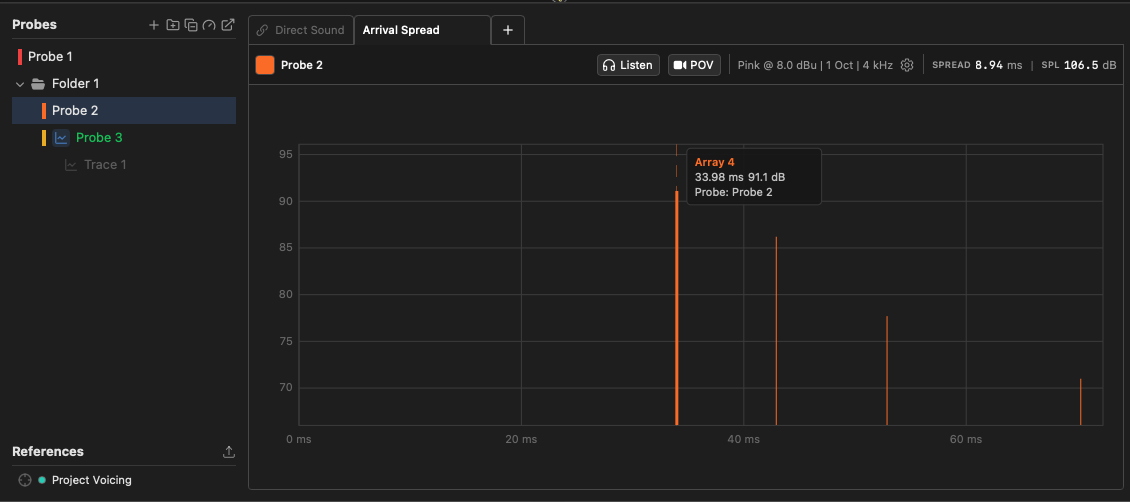
| Arrival Spread | Spread in arrival times of loudspeakers at the listener location. Indicates temporal smearing from multiple arrivals and reflections and the potential for echoes in large venues. | Echogram | |
(1) These parameters depended on the project containing a properly configured acoustical environment. In addition, the system considers the room acoustics behavior to be fully diffuse and uniform in nature for these parameters to reflect reality.
All parameters include the effects of air loss and propagation delay (controlled by project humidity and temperature settings).
SPL Modes
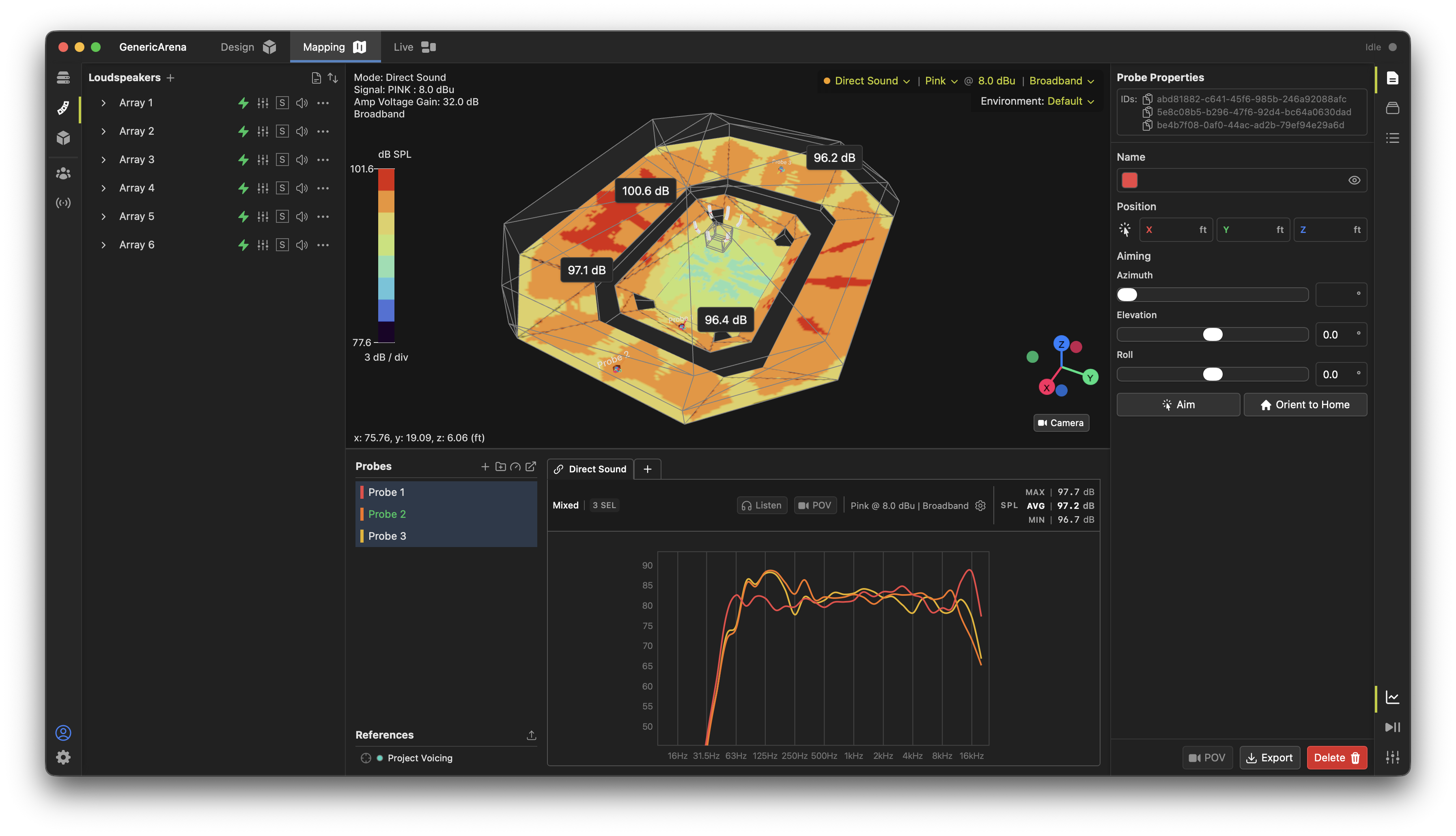
Direct Sound
The Direct Sound mode shows the energy contributed from each loudspeaker to the mapping area or probe with no contribution from room reflections. This is the same SPL behavior available in previous versions of Fulcrum One and serves as the baseline for evaluating system coverage and level. Because it ignores the room entirely, Direct Sound is the most reliable way to judge loudspeaker aiming, coverage uniformity, and the level relationships between sources. Use it early in a design to dial in physical placement and splay before layering in the room-dependent metrics.
Direct sound does include the effects of air loss and propagation delay based on the temperature and humidity settings in the project. The summation for Direct Sound is coherent (complex) in nature.
See Loudspeaker Coverage Mapping for more information.
Total SPL
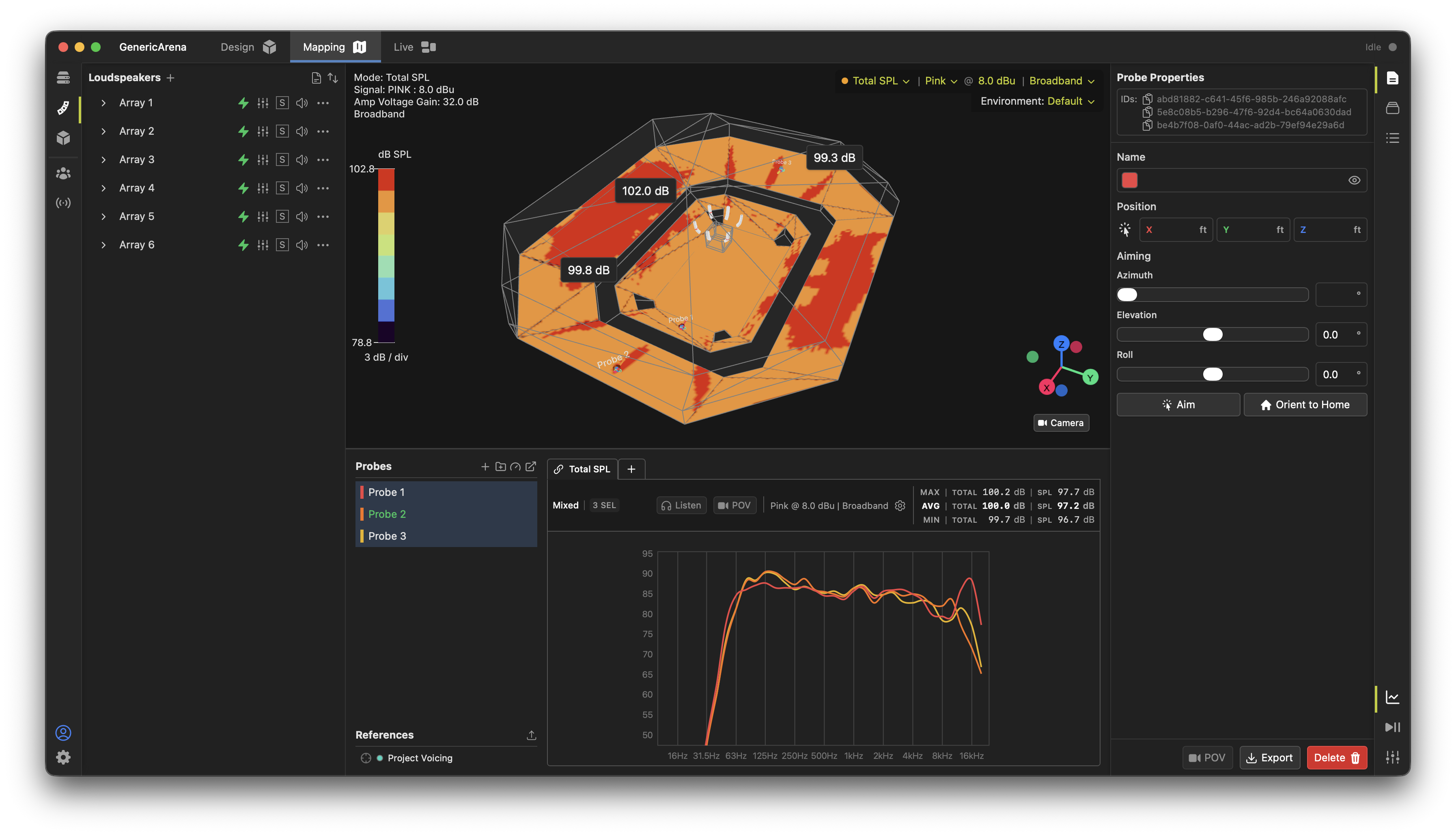
Total SPL combines the direct sound with the reverberant energy contributed by the room, giving the full sound pressure level a listener would experience at every location. This reflects how the space itself reinforces the system output and the total sound pressure level you can expect to achieve under the simulated conditions.
To obtain this value, the reverberant field intensity is computed based on the current environment and the sound power of each loudspeaker in the room (assuming a diffuse, statistical reverberant field). This intensity is added to the coherently-summed Direct Sound intensity at each location. The Total SPL sum does not include the ambient room noise, but only energy originating from the loudspeaker system.
Use Total SPL to verify the maximum output capability of the system in its installed environment, to check headroom against target levels, and to understand how much the room contributes to overall loudness. In highly reverberant spaces the difference between Direct Sound and Total SPL can be significant. This evaluation should be done in concert with quality metrics like STI or direct-to-reverberant ratio to qualify the result beyond overall level.
Compare the Total SPL result below to that of the example above to see a typical increase in SPL due to room effects, which can be very frequency-dependent in nature.
Ratio Modes
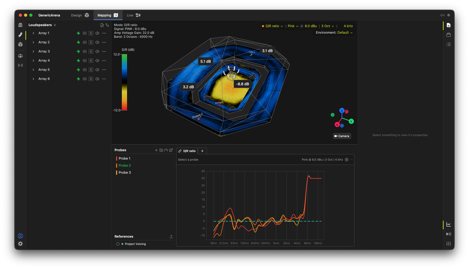
D/R Ratio
The Direct-to-Reverberant ratio expresses the level difference between the direct sound and the reverberant field. A higher D/R ratio means the direct sound dominates, which generally translates to a clearer, more immediate, and better-localized source.
To obtain this value, the reverberant field intensity is computed based on the current environment and the sound power of each loudspeaker in the room (assuming a diffuse, statistical reverberant field). This intensity is compared against the coherent direct sound summation at each location. The D/R ratio does not include the ambient room noise, but only energy originating from the loudspeaker system.
Use D/R Ratio to predict the perceived clarity and intimacy of the system in a reverberant space, to compare loudspeaker layouts that trade off coverage against directivity, and to identify areas where reflections may overwhelm the intended sound.
S/N Ratio
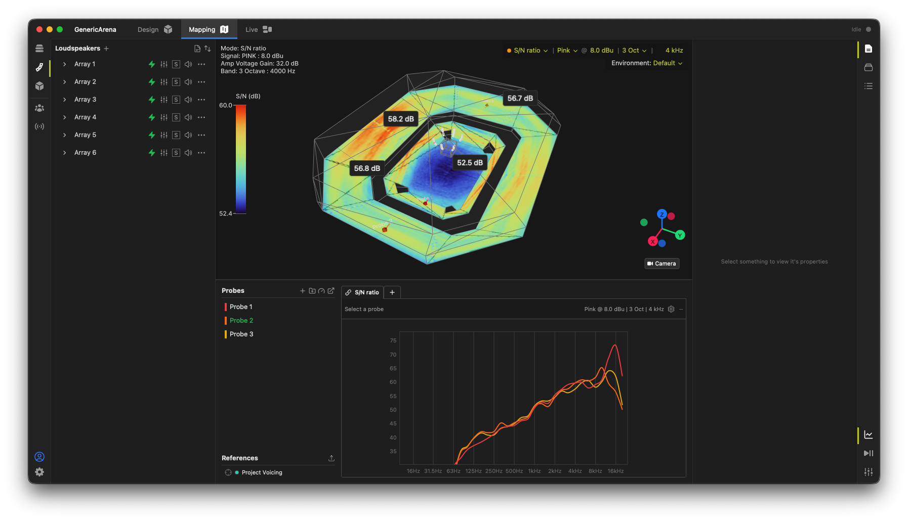
The Signal-to-Noise ratio compares the Total SPL of the system and room against the venue's background noise level. It indicates how far the program material rises above ambient noise at each location.
To obtain this value, the Total SPL is calculated per the method outlined above and compared against the ambient room noise at each location, assuming both the reverberation and room noise are statistically diffuse throughout the space.
Use S/N Ratio to gauge intelligibility and required output capacity in the presence of HVAC, crowd, or environmental noise, and to confirm that the system can deliver adequate level above the noise floor across the entire listening area.
Density
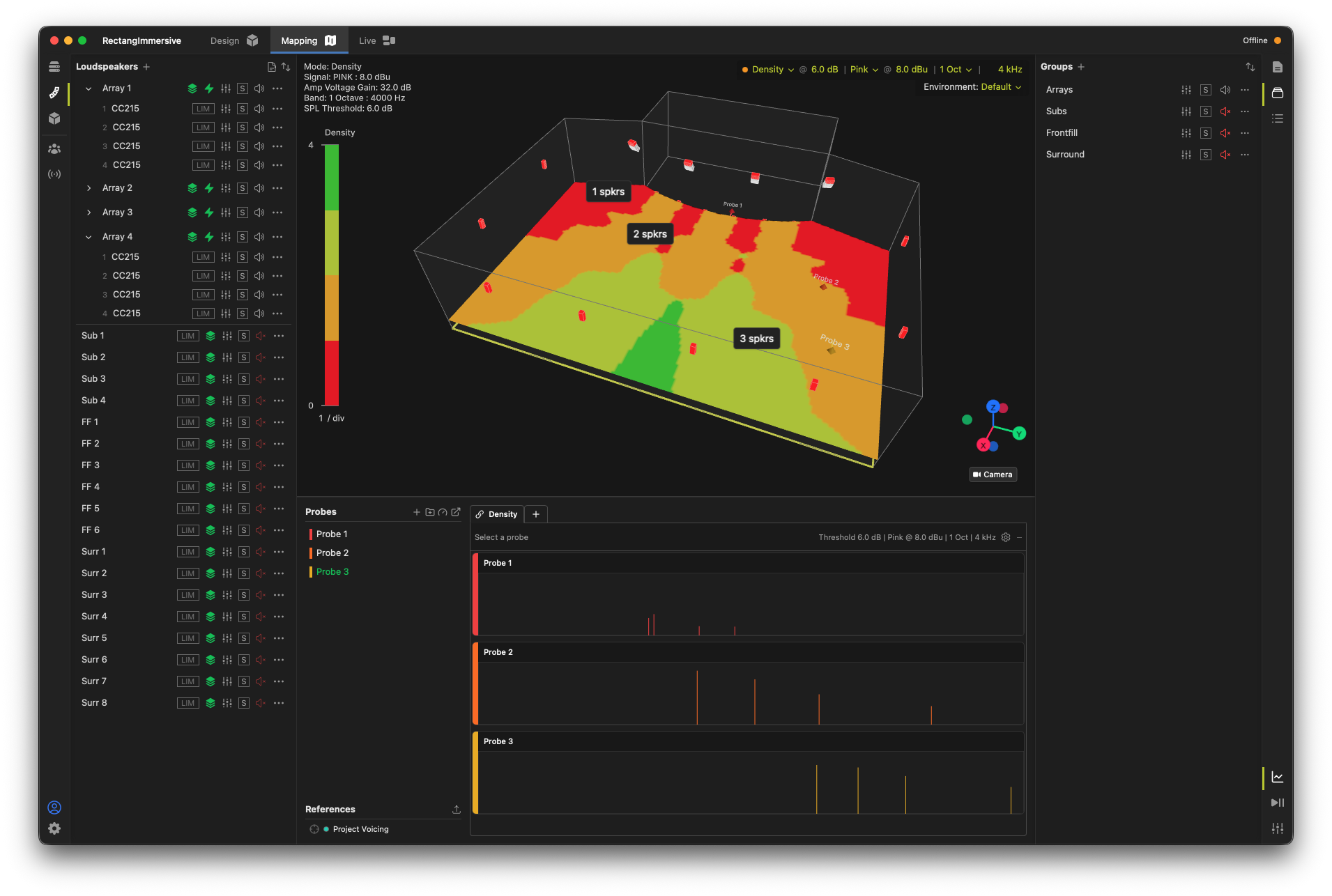
Density counts the number of loudspeakers audible at a location within a defined level threshold relative to the loudest loudspeaker at that location. It reveals how many sources are meaningfully contributing at each point in the coverage area. Set the threshold using the "@ dB" control in the mapping control pane:

Use Density to gauge overlap and redundancy in conventional systems, and to evaluate panning efficiency in immersive designs—where the number of contributing loudspeakers directly affects the precision and stability of spatial imaging. Any open Probes will show an echogram when using this mode, allowing you to further explore loudspeaker arrivals at probe locations.
STI
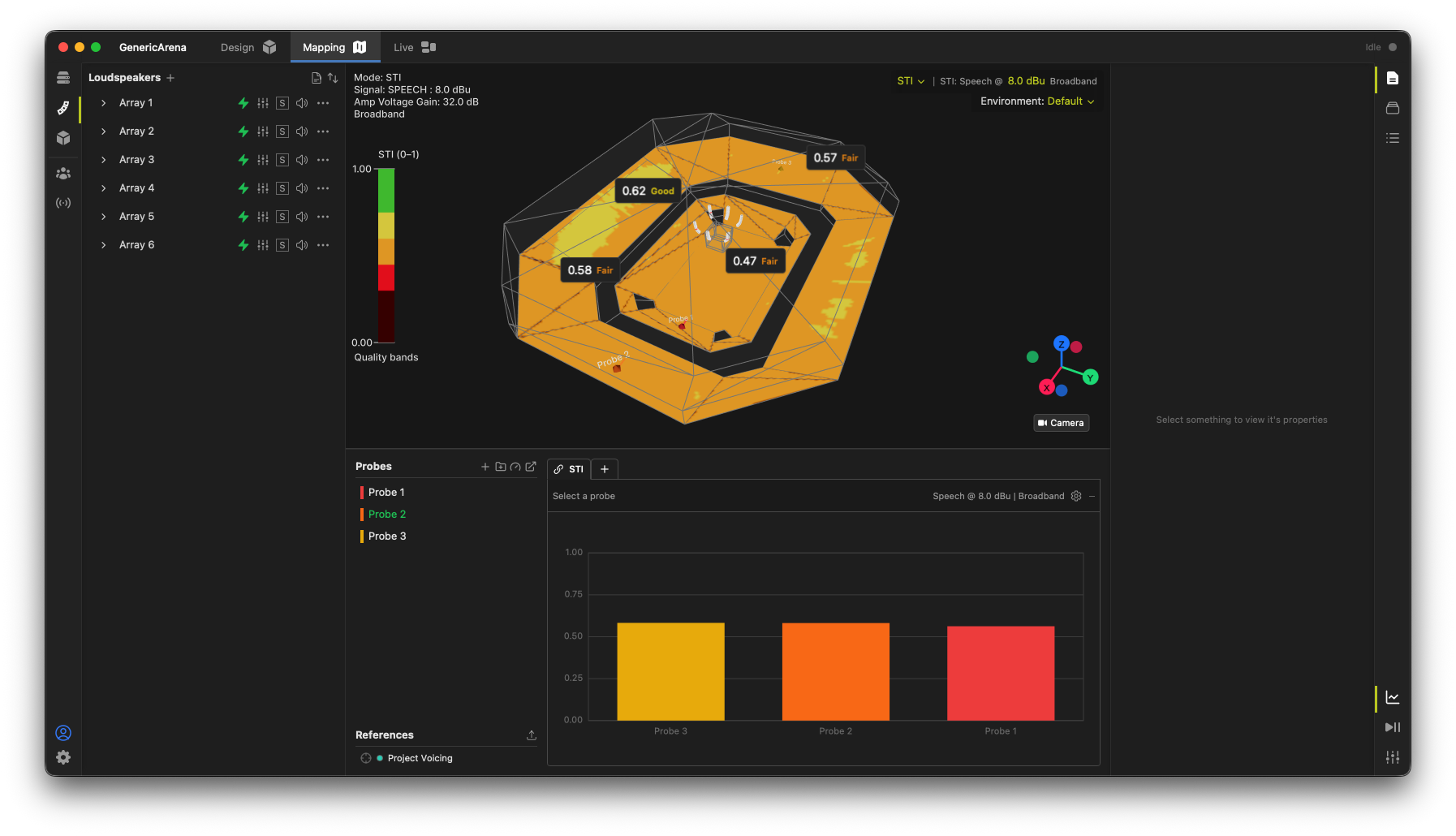
The Speech Transmission Index is a standardized metric on a 0–1 scale that predicts speech intelligibility, accounting for direct sound, reverberation, and background noise together. Higher values indicate clearer, more intelligible speech.
STI is computed based on the current environment settings for reverberation time and noise level, and evaluates these metrics against the direct sound at each mapping or probe location. The calculation adheres to IEC 60268-16:2020 using the Houtgast statistical method with a male speech signal. Note that this analysis ignores time-domain defects (echoes, system time alignment, etc.) and assumes the reverberant and noise fields are fully diffuse and isotropic.
By default, Fulcrum One displays the STI results in contour mode using the following categories as defined by IEC 60268-16:2020:
| STI Label Range | Standard STI |
|---|---|
| Bad | 0.0 - 0.30 |
| Poor | 0.30 - 0.45 |
| Fair | 0.45 - 0.60 |
| Good | 0.60 - 0.75 |
| Excellent | 0.75 - 1.00 |
Use STI to verify that announcements, paging, and speech content meet intelligibility requirements—including code-mandated thresholds for life-safety and voice-evacuation systems—and to target problem zones where reverberation or noise degrades clarity.
Timing Modes
Arrival (Earliest)
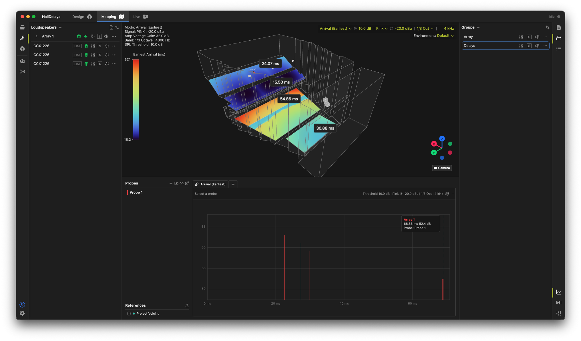
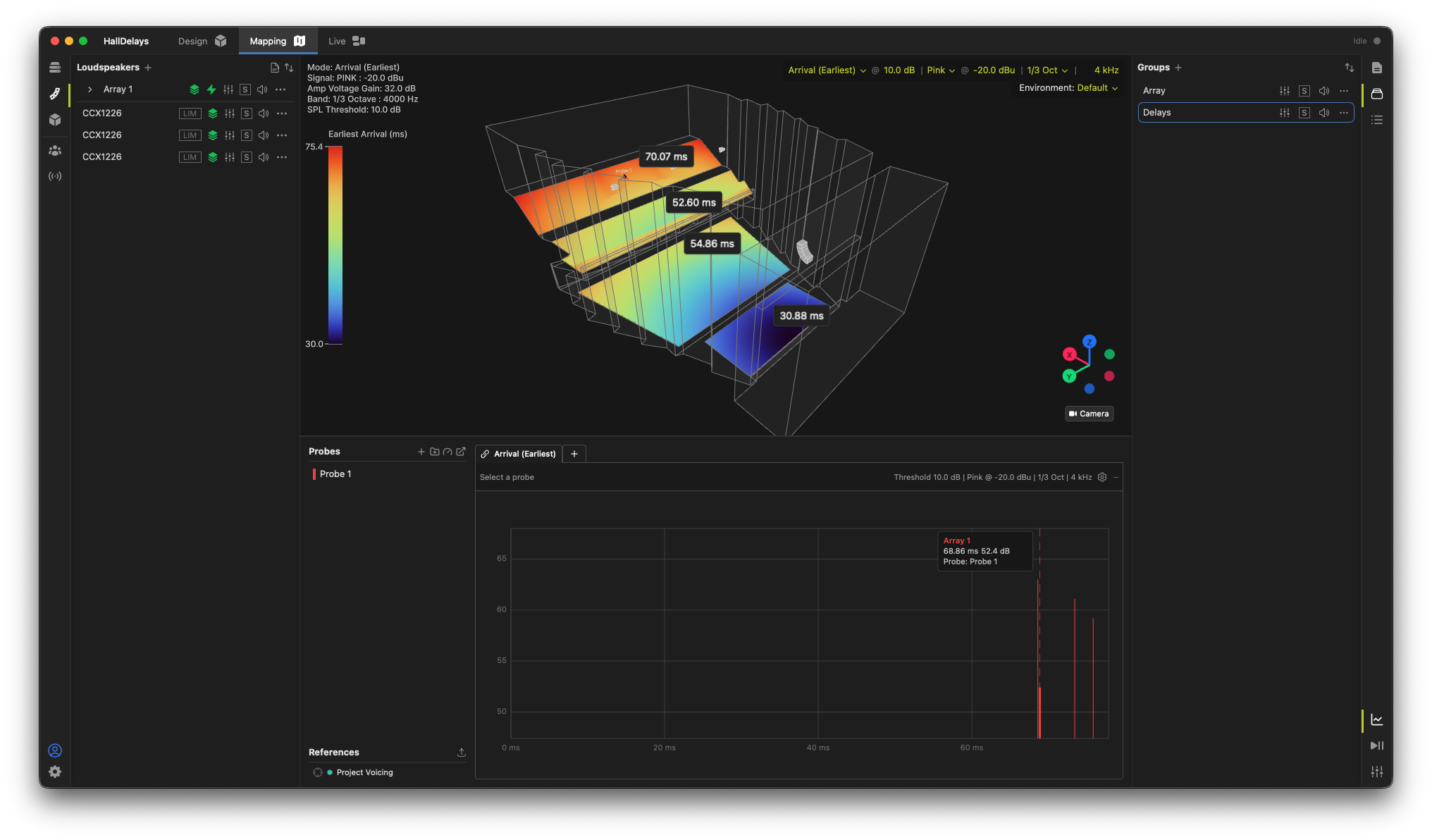
Arrival (Earliest) reports the arrival time of the first loudspeaker to reach each listener location within a defined level threshold relative to the loudest loudspeaker at that location. It maps how sound propagates through the space from the nearest contributing source. Set the threshold relative to the loudest arrival using the "@ dB" control in the mapping control pane:

Use this parameter to set delay times, to verify time alignment across zones and fills, and to ensure that the intended source arrives first so that localization and front-to-back imaging behave as designed.
Arrival Spread
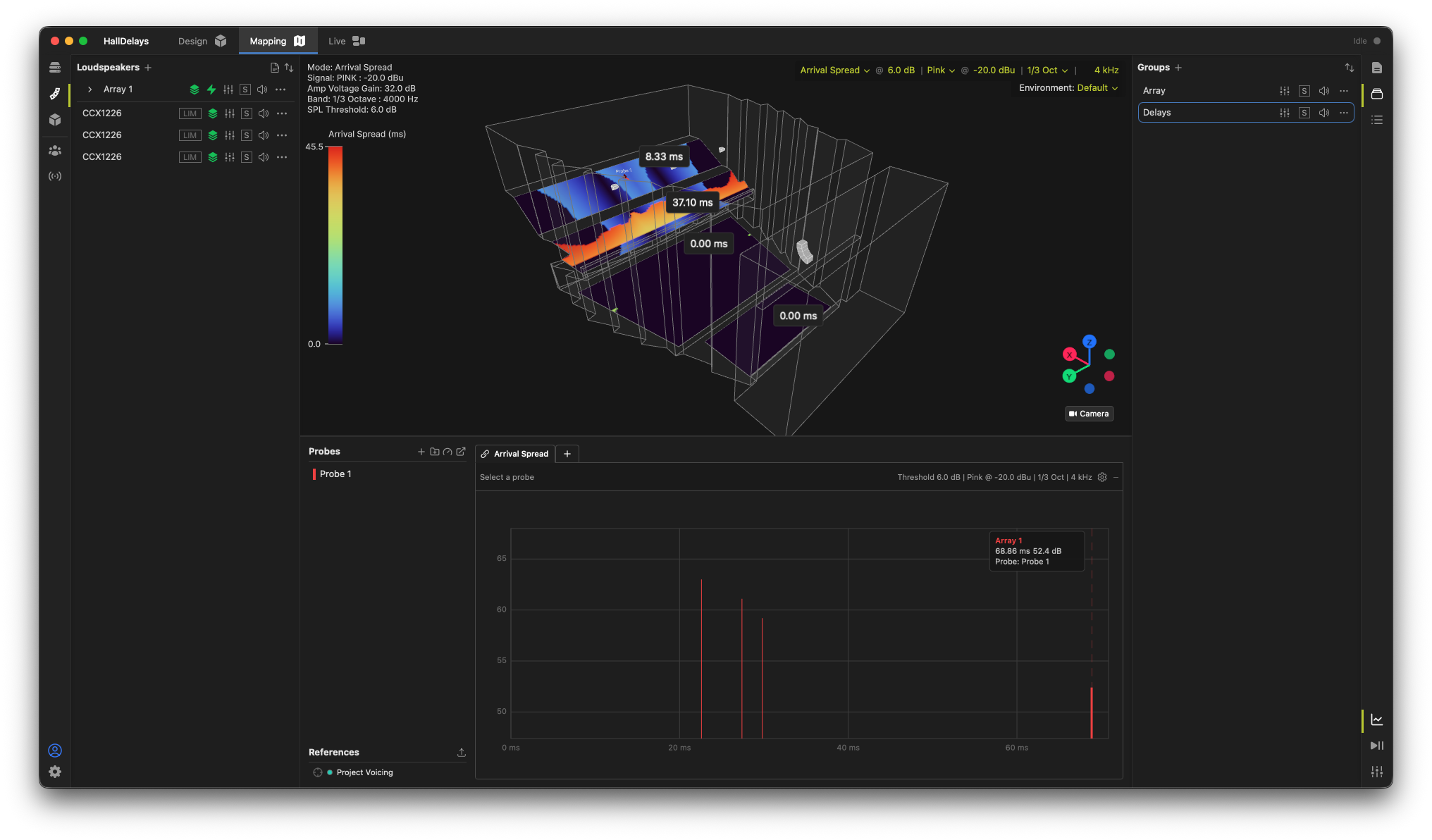
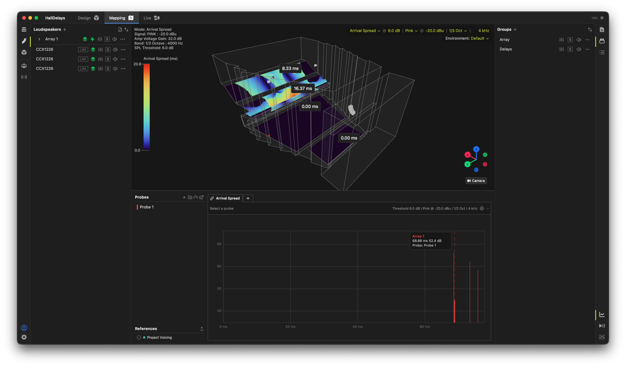
Arrival Spread shows the range of arrival times from all loudspeakers contributing at a given location. A wide spread indicates temporal smearing caused by multiple arrivals.
Set the threshold using the "@ dB" control in the mapping control pane:

Use Arrival Spread to identify regions prone to echoes or comb filtering, particularly in large venues with many overlapping sources, and to refine delay and coverage decisions that tighten the system's temporal response.
Room Auralization
Room Auralization lets you hear your loudspeaker design over a pair of headphones, rendered binaurally from the position of a mapping probe and including the reverberation of the active environment. It is the audible counterpart to the simulation modes: where the map shows you the numbers, Room Auralization Mode lets you listen to the result from any seat in the venue.
To start, select a single probe and press
Quickstart
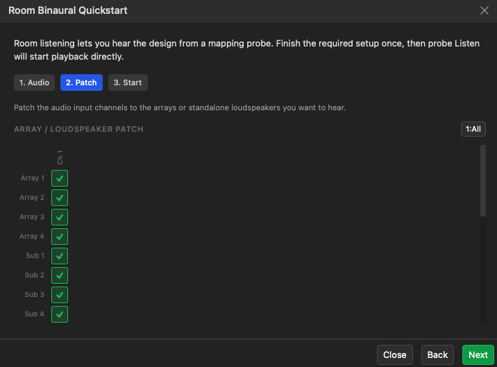
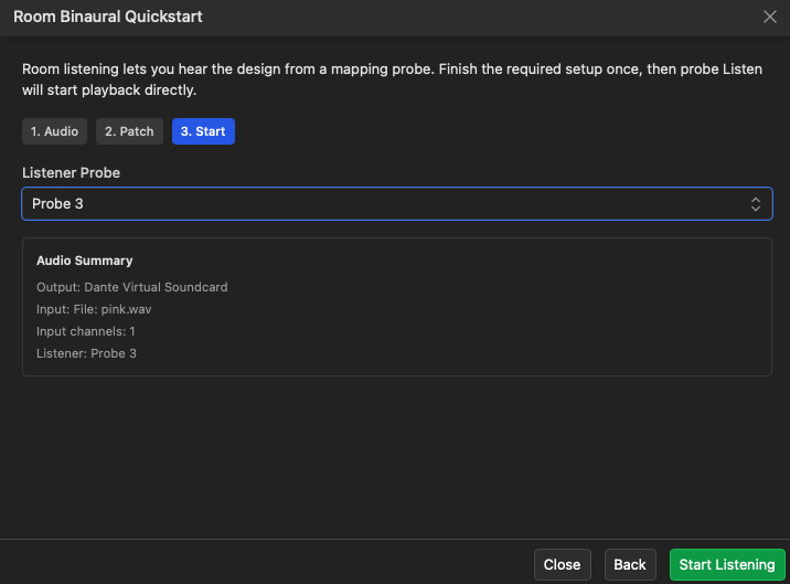
The first time you listen, a short Room Binaural Quickstart wizard walks you through the required setup. Once it is complete, the probe Listen button starts playback directly.
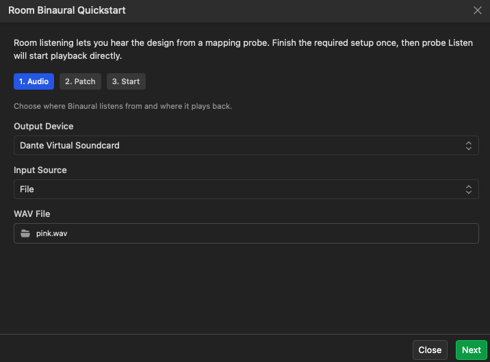
- Audio — choose the output device for your headphones and the input source. The input can be a live audio device or a WAV file (such as a piece of program material).
- Patch — route the input channels to the arrays and standalone loudspeakers you want to hear. Use 1:All to send a single input channel to every loudspeaker at once.
- Start — pick the Listener Probe to render from and review the audio summary before you begin.
Playback and Head Tracking
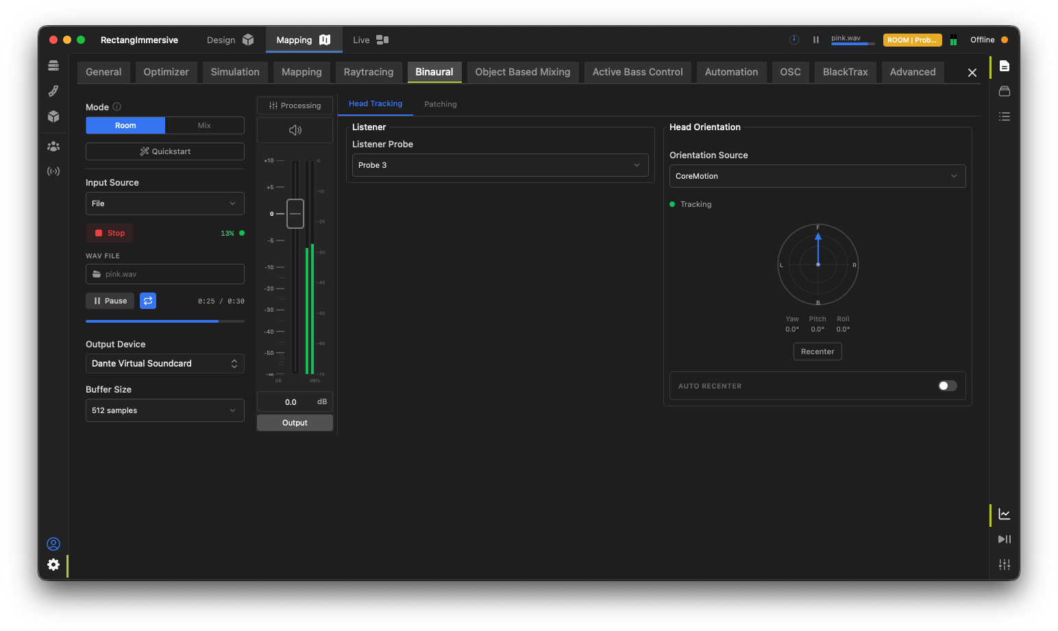
While listening, the Binaural Playback panel provides transport controls, output device and listener-probe selection, an output level, and a level meter.
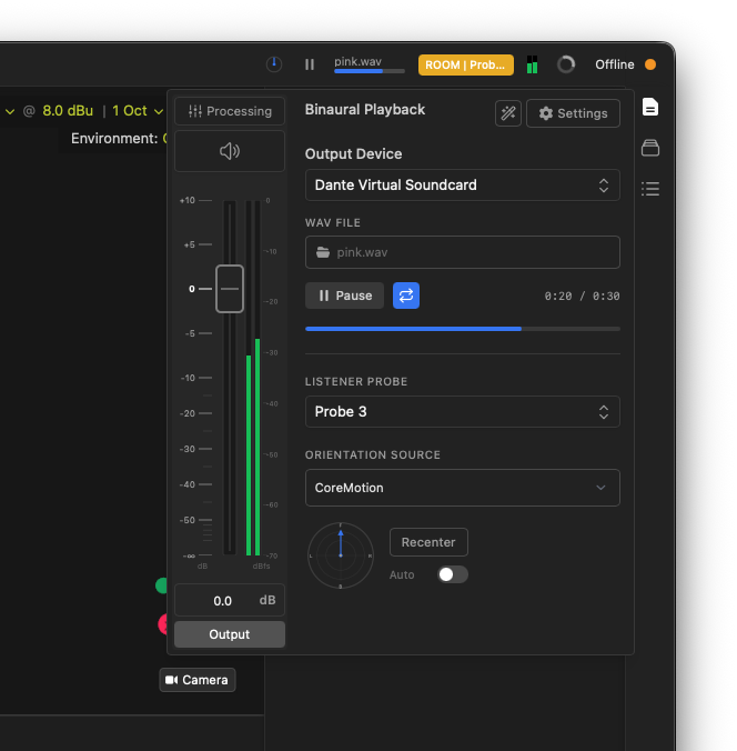
The Orientation Source controls how the listener's head orientation is determined. Choose Manual to set the yaw/pitch/roll by hand (or by clicking and dragging the POV camera in the 3D view), or CoreMotion to track supported Apple headphones directly on a Mac (see Binaural Head Tracking). Head tracking is optional—you can position and orient the listener entirely by hand. Use Recenter to make the current head position the new forward reference, and enable Auto Recenter to do so automatically after a set period of stillness.
Click the Settings cog to see additional settings for Room Auralization Mode in the Binaural submenu.